Tutorial: AutoAI multivariate time series experiment with Supporting features
Use sample data to train a multivariate time series experiment that predicts pollution rate and temperature with the help of supporting features that influence the prediction fields.
When you set up the experiment, you load sample data that tracks weather conditions in Beijing from 2010 to 2014. The experiment generates a set of pipelines that use algorithms to predict future pollution and temperature with supporting features, including dew, pressure, snow, and rain. After generating the pipelines, AutoAI compares and tests them, chooses the best performers, and presents them in a leaderboard for you to review.
Data set overview
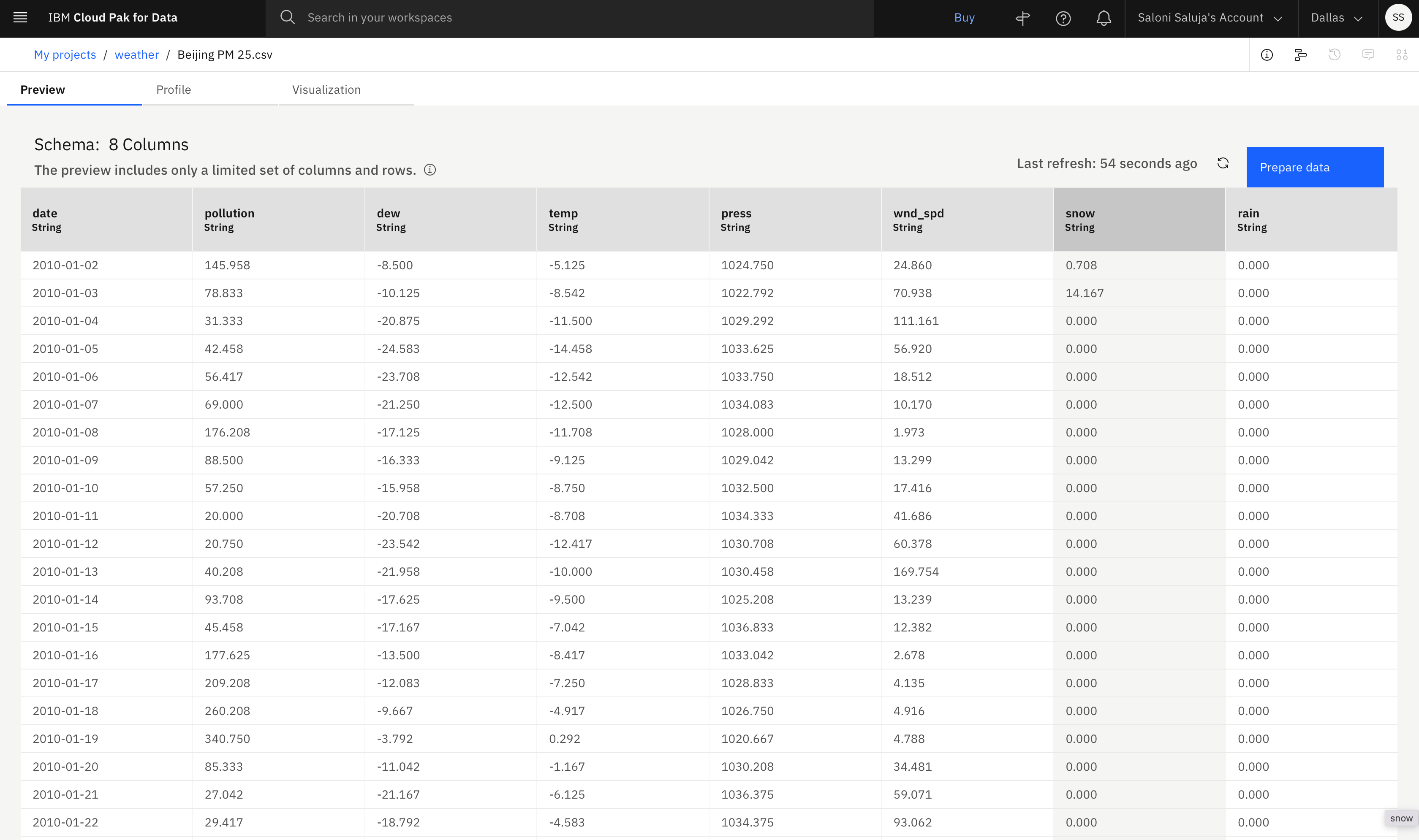
For this tutorial, you use the Beijing PM 2.5 data set from the Resource hub. This data set describes the weather conditions in Beijing from 2010 to 2014, which are measured in 1-day steps, or increments. You use this data set to configure your AutoAI experiment and select Supporting features. Details about the data set are described here:
- Each column, other than the date column, represents a weather condition that impacts pollution index.
- The Resource hub entry shows the origin of the data. You can preview the file before you download the file.
- The sample data is structured in rows and columns and saved as a .csv file.
Tasks overview
In this tutorial, you follow steps to create a multivariate time series experiment that uses Supporting features:
Create a project
Follow these steps to create an empty project and download the Beijing PM 2.5 data set from the IBM watsonx Resource hub:
- From the main navigation pane, click Projects > View all projects, then click New Project.
a. Click Create an empty project.
b. Enter a name and optional description for your project.
c. Click Create. - From the main navigation panel, click Resource hub and download a local copy of the Beijing PM 2.5 data set.
Create an AutoAI experiment
Follow these steps to create an AutoAI experiment and add sample data to your experiment:
-
On the Assets tab from within your project, click New asset > Build machine learning models or Retrieval-augmented generation patterns automatically.
-
Specify a name and optional description for your experiment.
-
Associate a machine learning service instance with your experiment.
-
Choose an environment definition of 8 vCPU and 32 GB RAM.
-
Click Create.
-
To add sample data, choose one of the these methods:
- If you downloaded your file locally, upload the training data file, PM25.csv by clicking Browse and then following the prompts.
- If you already uploaded your file to your project, click Select from project, then select the Data asset tab and choose Beijing PM 25.csv.
Configure the experiment
Follow these steps to configure your multivariate AutoAI time series experiment:
-
Click Yes for the option to create a Time Series Forecast.
-
Choose as prediction columns:
pollution,temp. -
Choose as the date/time column:
date.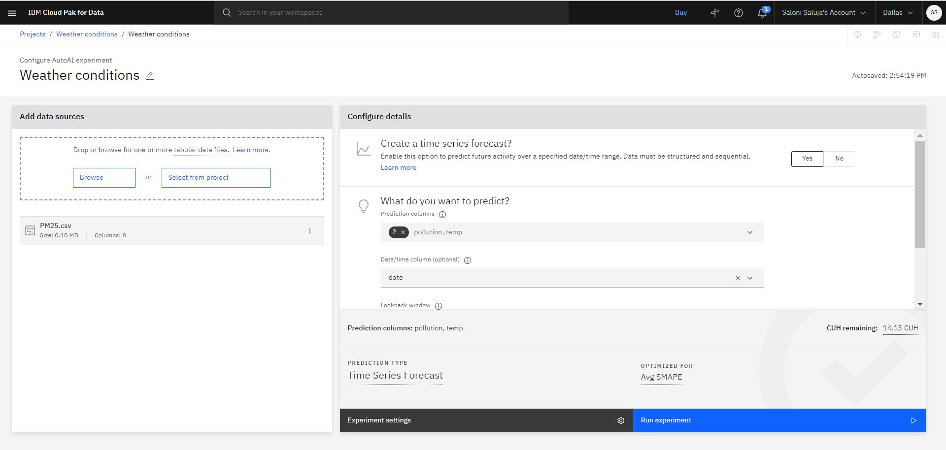
-
Click Experiment settings to configure the experiment:
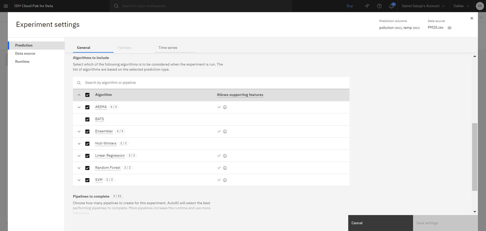
a. In the Prediction page, accept the default selection for Algorithms to include. Algorithms that allow you to use Supporting features are indicated by a checkmark in the column Allows supporting features.
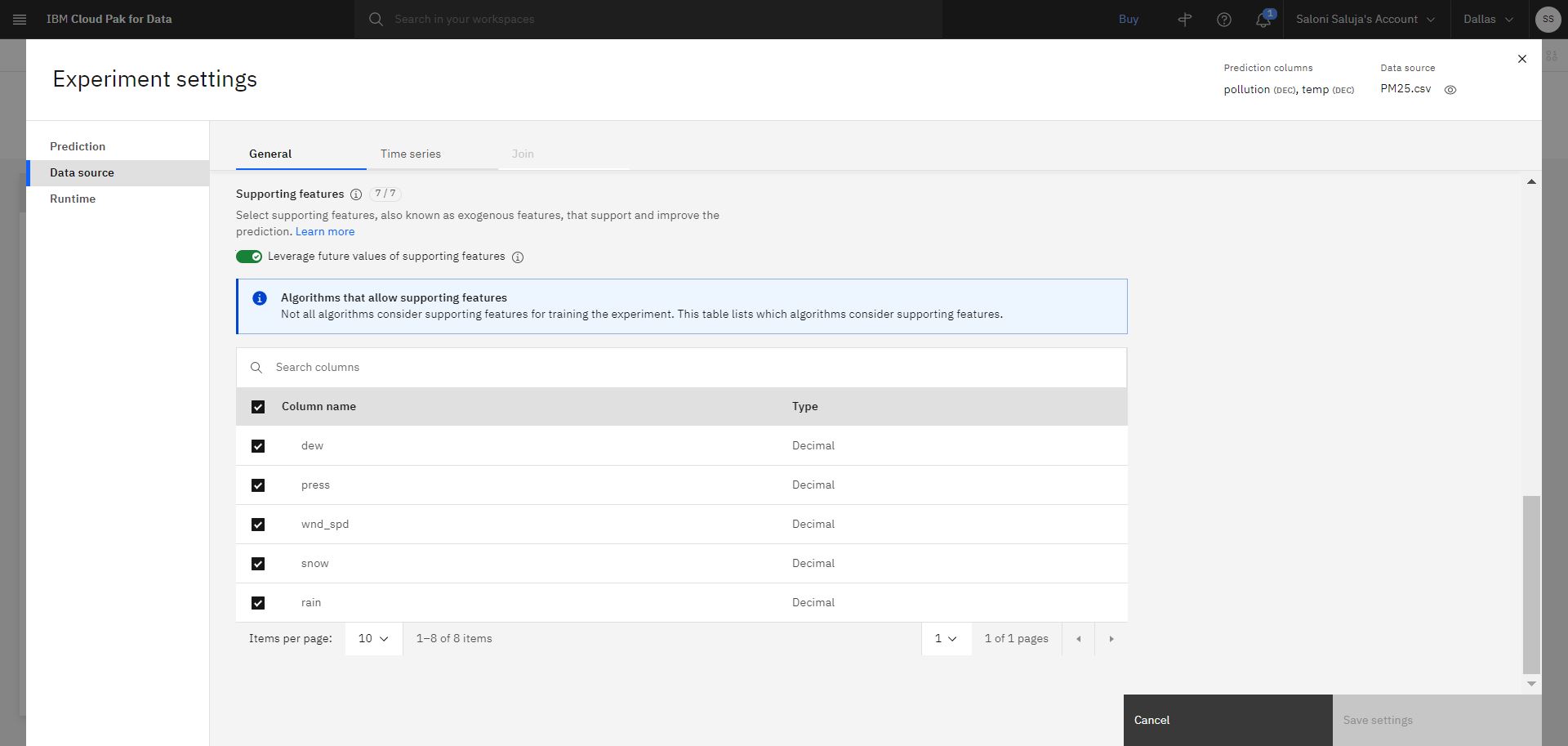
b. Go to the Data Source page. For this tutorial, you will supply future values of Supporting features while testing. Future values are helpful when values for the supporting features are knowable for the prediction horizon. Accept the default enablement for Leverage future values of supporting features. Additionally, accept the default selection for columns that will be used as Supporting features.
c. Click Cancel to exit from Experiment settings. -
Click Run experiment to begin the training.
Review experiment results
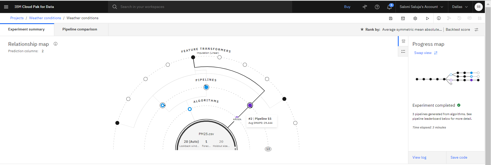
The experiment takes several minutes to complete. As the experiment trains, the relationship map shows the transformations that are used to create pipelines. Follow these steps to review experiment results and save the pipeline with the best performance.
-
Optional: Hover over any node in the relationship map to get details on the transformation for a particular pipeline.
-
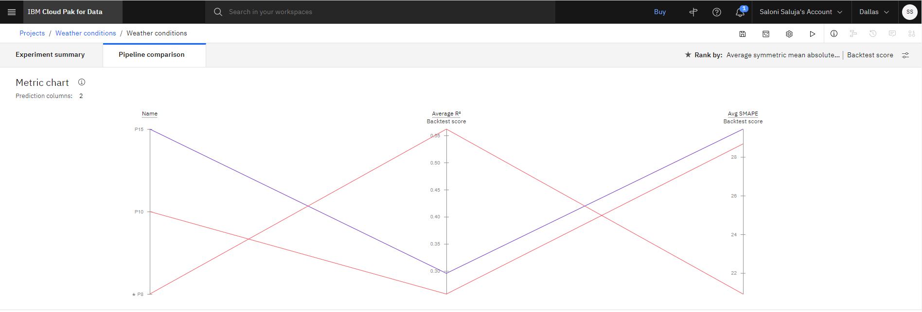
Optional: After the pipelines are listed on the leaderboard, click Pipeline comparison to see how they differ. For example:
-
When the training completes, the top three best performing pipelines are saved to the leaderboard. Click any pipeline name to review details.
Note: Pipelines that use Supporting features are indicated by **SUP** enhancement.
-
Select the pipeline with Rank 1 and click Save as to create your model. Then, click Create. This action saves the pipeline under the Models section in the Assets tab.
Deploy the trained model
Before you can use your trained model to make predictions on new data, you must deploy the model. Follow these steps to promote your trained model to a deployment space:
- You can deploy the model from the model details page. To access the model details page, choose one of these options:
- Click the model’s name in the notification that is displayed when you save the model.
- Open the Assets page for the project that contains the model and click the model’s name in the Machine Learning Model section.
- Click the Promote to deployment space
icon, then select or create a deployment space where the model will be deployed.
Optional: Follow these steps to create a deployment space:
a. From the Target space list, select Create a new deployment space.
b. Enter a name for your deployment space.
c. To associate a machine learning instance, go to Select machine learning service (optional) and select a machine learning instance from the list.
d. Click Create. - Once you select or create your space, click Promote.
- Click the deployment space link from the notification.
- From the Assets tab of the deployment space:
a. Hover over the model’s name and click the deployment icon .
.
b. In the page that opens, complete the fields:
- Select Online as the Deployment type.
- Specify a name for the deployment.
- Click Create.
After the deployment is complete, click the Deployments tab and select the deployment name to view the details page.
Test the deployed model
Follow these steps to test the deployed model from the deployment details page:
-
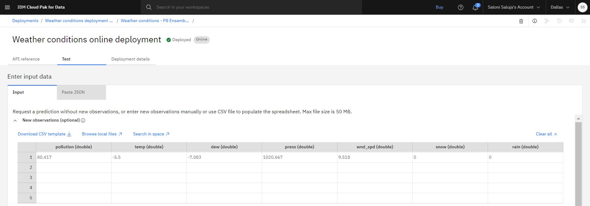
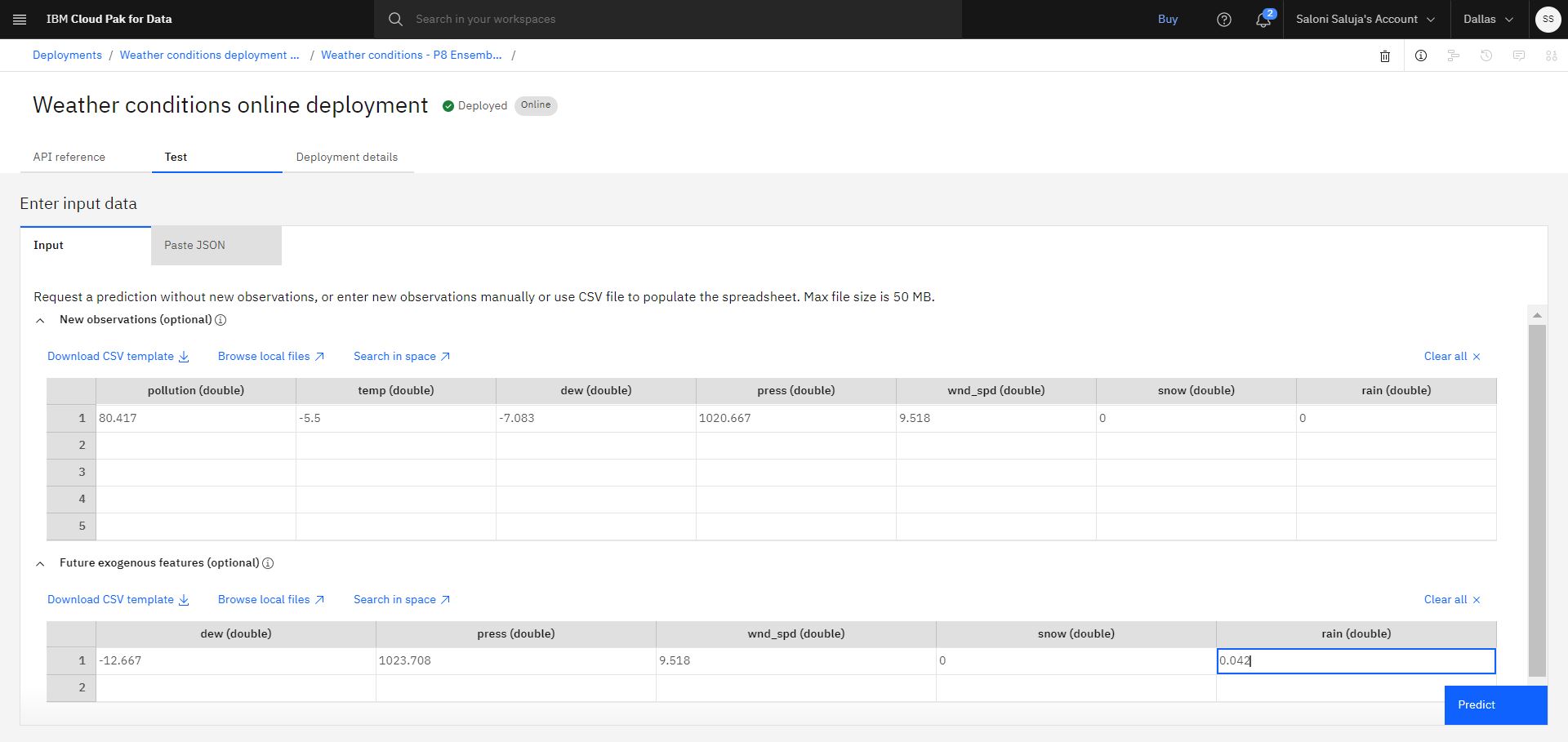
On the Test tab of the deployment details page, go to New observations (optional) spreadsheet and enter the following values:
pollution (double):80.417
temp (double):-5.5
dew (double):-7.083
press (double):1020.667
wnd_spd (double):9.518
snow (double):0
rain (double):0 -
To add future values of Supporting features, go to Future exogenous features (optional) spreadsheet and enter the following values:
dew (double):-12.667
press (double):1023.708
wnd_spd (double):9.518
snow (double):0
rain (double):0.042Note: You must provide the same number of values for future exogenous features as the prediction horizon that you set during experiment configuration stage. -
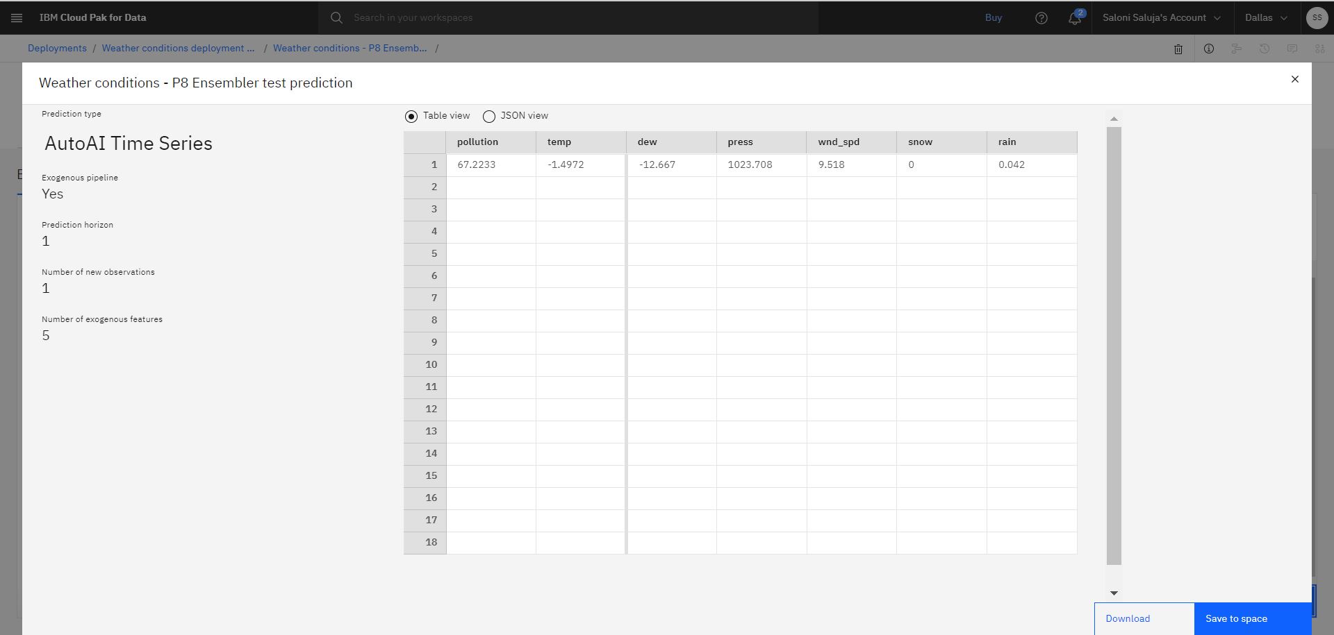
Click Predict. The resulting prediction indicates values for pollution and temperature.
Note: Prediction values that are shown in the output might differ when you test your deployment.
Learn more
Parent topic: Building a time series experiment
